Finite Volume Methods for Simulating Fluid Flows
Undergraduate Project 2025-26 (3H)
Finite difference methods offer a simple and intuitive approach to solving partial differential equations: by replacing derivatives with algebraic approximations, they transform continuous problems into solvable systems of equations. (It’s hard to find a clearer overview of finite difference schemes than the one on Wikipedia!) However, this simplicity comes with a major limitation: finite difference methods do not inherently respect the physical conservation laws—mass, momentum, and energy—that govern fluid dynamics.
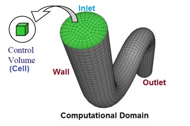
That’s where the strength of finite volume methods (FVM) truly shines. Rather than approximating derivatives at isolated points, FVM partitions the computational domain into a mosaic of control volumes (or cells, as shown in the figure below), with each volume treated as a small, self-contained system. Within each cell, the conservation laws are applied directly in their integral form, ensuring that the fluxes entering and leaving are consistently balanced. This means every quantity is accounted for—nothing is artificially gained or lost—which is crucial when simulating realistic physical systems.
Another major advantage of FVM lies in its flexibility with complex geometries. Take the flow in the twisted pipe shown below: it’s difficult to lay down a regular grid for finite difference approximations. But with FVM, we don’t need to force a regular structure. Instead, we work with irregularly shaped cells and apply local rules for each, allowing the method to adapt naturally to the geometry of the problem.
More philosophically, FVM teaches a mindset every scientist can have: think in fluxes, think in balances, think in guarantees. Whether you’re simulating the spin-up of a tropical cyclone or the migration of a planetary jet, the method quietly reinforces the principle:“Honor what nature refuses to break, and your simulation will carry the truth farther than you dreamed.” That’s why finite volume methods feel less like a numerical workaround and more like a pact with the laws of physics—and once you’ve experienced that clarity, it’s hard to go back. In this project, we will learn the foundations and key variations of finite volume methods and apply them to model a range of fluid flows.
More philosophically, FVM teaches a mindset every scientist can have: think in fluxes, think in balances, think in guarantees. Whether you’re simulating the spin-up of a tropical cyclone or the migration of a planetary jet, the method quietly reinforces the principle:“Honor what nature refuses to break, and your simulation will carry the truth farther than you dreamed.” That’s why finite volume methods feel less like a numerical workaround and more like a pact with the laws of physics—and once you’ve experienced that clarity, it’s hard to go back. In this project, we will learn the foundations and key variations of finite volume methods and apply them to model a range of fluid flows.
This project is co-supervised by Hossein Kafiabad and Cai Maitland-Davies, and it involves substantial programming and a strong interest in fluid simulation. It is recommended that you take Fluid III concurrently, and some background in numerical methods will be an asset.
[1] Watching this video give you a general picture of FVM:
[2] This book is one of the to go references for FVM: Versteeg, H. K., and W. Malalasekera. “Computational fluid dynamics.” The finite volume method (1995): 1-26.